13.4 Notes on estimating measurement uncertainty due to linear regression

Questions about handling linear regression in measurement uncertainty estimation have over the years come up quite often in these courses. The way we see it, there are in very broad terms four approaches, how one can estimate measurement uncertainty when linear regression is involved. Three of them, with different levels of rigor, are based on modeling. The fourth is based on validation and quality control data.

1. Modeling-based approaches

The main common advantages and disadvantages of the model-based approaches are as follows:

The advantages of these approaches are that they enable us to assign uncertainties to all influencing parameters naturally account for all uncertainty sources; if the uncertainty sources have been realistically quantified then the uncertainty budget enables seeing the individual contributions of all uncertainty sources.

The disadvantages are that the model must enable us to account for all uncertainty sources and reliable quantitative estimates have to exist for all of them. Obtaining these estimates may be difficult in complex chemical analysis (especially the ones related to analyte losses during sample preparation, possible interferences, etc) and may need significant additional work. If some uncertainty source is overlooked or not adequately quantified then these approaches can lead to serious underestimating of uncertainty. The calculations can be quite complex and there is a danger of making mistakes.

The specific advantages and disadvantages of the individual approaches are presented below.

1.1 The “full approach”

This approach looks at all the operations in the method and quantifies their uncertainty sources. In particular, for evaluating the uncertainty due to linear regression, this approach takes into account the uncertainties involved in preparation of the calibration solutions, as well as the uncertainties of the measured signals. Correlation between slope and intercept is accounted for in the model starts from the preparation of the stock solution and then diluting it. Scatter of data points around the calibration line is accounted for by their individual uncertainties, not by statistical analysis of the regression.

An example of this approach, applied to the example presented in Section 9 of the course – determination of ammonium nitrogen in water – can be found at https://akki.ut.ee/GUM_examples/. See the example “Ammonium by Photometry”, elaboration level “High”.

The advantage is that the correlation between slope and intercept can be automatically accounted for (slope and intercept act as interim quantities, not as input quantities).

In order to account for the correlation between slope and intercept the measurement model has to start from preparing the stock solution that is thereafter diluted.

1.2 The “Eurachem approach”

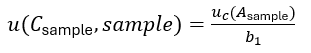
This is the approach quoted by Miguel. I call it here Eurachem approach because it is the approach presented in Appendix E.4 of the Eurachem uncertainty guide. I am presenting the corresponding equations here in slightly different form, which may be more convenient for you to use. The uncertainty of the analyte concentration in the sample, C_sample, can be expressed as follows:

,                (1)

where the first term           

 (2)

expresses the uncertainty originating from the measurement of the signal (e.g. photometric absorbance of peak area on a chromatogram) of the sample solution A_sample. This term is the one that has to account for uncertainty sources such as possible interferences, matrix effect, incomplete extraction of analyte from sample, etc. The middle term

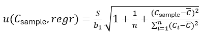                                                       (3)

expresses the uncertainty originating from the scatter of data points around the calibration line. S is the so-called linear regression standard deviation: 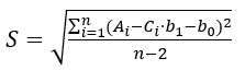                                                                            (4)

where n is the number of points on the regression line, C_i and A_i are the concentration and signal of the i-th calibration point,  is the arithmetic mean of the concentrations C_i and C_sample is the analyte concentration of the sample solution. S can be easily found using the LINEST function of the spreadsheet software. C_stock is the concentration of the stock solution and u(C_stock) is its standard uncertainty.

The last term in eq (1) is meant to take into account for uncertainty sources that affect all calibration points in a systematic way – i.e. without causing scatter. This term can be used e.g. for accounting for uncertainty of purity of standard substance that was used to make the calibration solutions.

Correlation between slope and intercept is automatically accounted for (uncertainties of slope and intercept are not included explicitly). Scatter of points around the regression line is explicitly accounted for.

The equations presented above are quite complex and there is a danger of making mistakes.

1.3 The “simplified approach”

This is the approach used in example presented in Section 9 of the course – determination of ammonium nitrogen in water. Explanations can be found in that section.

The advantages of this approach are that it is simpler to understand and use than the two previous approaches, yet all uncertainty sources can be accounted for.

The main disadvantage of this approach is that it ignores the negative correlation between slope and intercept of the calibration line with the consequence that the uncertainty gets somewhat overestimated (see the footnote in Section 9.5).

2. The Single-lab validation approach

This approach differs fundamentally from the model-based approaches in that linear regression is not specifically addressed at all in uncertainty calculations. The whole uncertainty evaluation is based on analysis results obtained with control samples (typically from control charts) and samples with known reference values of analyte concentrations (typically certified reference materials or spiked samples). This approach is explained in detail in Section 10 of this course.

The advantages of this approach are that it is a lot simpler to use than any of the modeling approaches and gives very realistic uncertainty estimates also for complex analysis methods (the danger to underestimate the uncertainty is low).

The main disadvantages of this approach are that it does not give information on the contributions of individual uncertainty sources and that a significant amount of validation data is needed and if this is not available, then it is not possible to use this approach.