
Brief summary: This section explains that whether an effect will influence the measurement result as a random or as a systematic effect depends on the conditions. Effects that are systematic in short term can become random in long term. This is the reason why repeatability is by its value smaller than within-lab reproducibility and the latter is in turn smaller than the combined standard uncertainty. This section also explains that the A and B type uncertainty estimates do not correspond one to one to the random and systematic effects.
How a within-day systematic effect can become a long-term random effect?
http://www.uttv.ee/naita?id=17713
https://www.youtube.com/watch?v=qObLSS7mfDo
Random and systematic effects in the short term and in the long term
An effect that within a short time period (e.g. within a day) is systematic can over a longer time period be random. Examples:
- If a number of pipetting operations are done within a day using the same pipette then the difference of the actual volume of the pipette from its nominal volume (i.e. calibration uncertainty) will be a systematic effect. If pipetting is done on different days and the same pipette is used then it is also a systematic effect. However, if pipetting is done on different days and different pipettes are used then this effect will change into a random effect.
- An instrument is calibrated daily with calibration solutions made from the same stock solution, which is remade every month. In this case the difference of the actual stock solution concentration and its nominal concentration is a systematic effect within a day and also within few weeks. But over a longer time period, say, half a year [1]It cannot be strictly defined, how long is „long-term“. An approximate guidance could be: one year is good, „several months“ (at least 4-5) is minimum. Of course it also depends on the procedure. . It cannot be strictly defined, how long is „long-term“. An approximate guidance could be: one year is good, „several months“ (at least 4-5) is minimum. Of course it also depends on the procedure. this effect becomes random, since a number of different sock solutions will have been in use during that time period.
Conclusions:
- An effect, which is systematic in short term can be random in long term;
- The longer is the time frame the more effects can change from systematic into random.
As explained in a past lecture if the measurement of the same or identical sample is repeated under identical conditions (usually within the same day) using the same procedure then the standard deviation of the obtained results is called repeatability standard deviation and denoted as sr. If the measurement of the same or identical sample is repeated using the same procedure but under changed conditions whereby the changes are those that take place in the laboratory under normal work practices then the standard deviation of the results is called within-lab reproducibility or intermediate precision and it is denoted as sRW. [2][2] The terms „within-lab reproducibility“ and „intermediate precision“ are synonyms. The VIM(1) prefers intermediate precision. The Nordtest handbook(5) uses within-lab reproducibility (or reproducibility within laboratory). In order to stress the importance of the „long-term“, in this course we often refer to sRW as the within-lab long-term reproducibility.
The conclusions expressed above are the reason why sr is smaller than sRW. Simply, some effects that within day are systematic and are not accounted for by sr become random over a longer time and sRW takes them into account. The combined standard uncertainty uc is in turn larger that the intermediate precision, because it has to take into account all significant effects that influence the result, including those that remain systematic also in the long term. This important relation between these three quantities is visualized in Scheme 6.1.
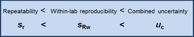
Scheme 6.1. Relations between repeatability, within-lab reproducibility and combined uncertainty.
The random and systematic effects cannot be considered to be in one-to-one relation with type A and B uncertainty estimation. These are categorically different things. The effects refer to the intrinsic causal relationships, while type A and B uncertainty estimation refers rather to approaches used for quantifying uncertainty. Table 6 illustrates this further.
Table 6.1. Interrelations between random and systematic effects and A and B types of uncertainty estimates.
|
Effect |
Type A estimation |
Type B estimation |
|
Random |
The usual way of estimating uncertainties caused by random effects |
Type B estimation of the uncertainty caused by random effects is possible if no repeated measurements are carried out and the data/information on the magnitude of the effect is instead available from different sources. |
|
Systematic |
This is only possible if the effect will change into a random effect in the long term |
The usual way of estimating uncertainties caused by the systematic effects |
So, depending on the timeline, all the effects causing uncertainty can be grouped as pictured in Scheme 6.2. In the short-term view, most effects act as systematic and the random effects can be quantified via repeatability. In the long term more (usually most) effects are random and can be quantified via within-lab reproducibility (intermediate precision).
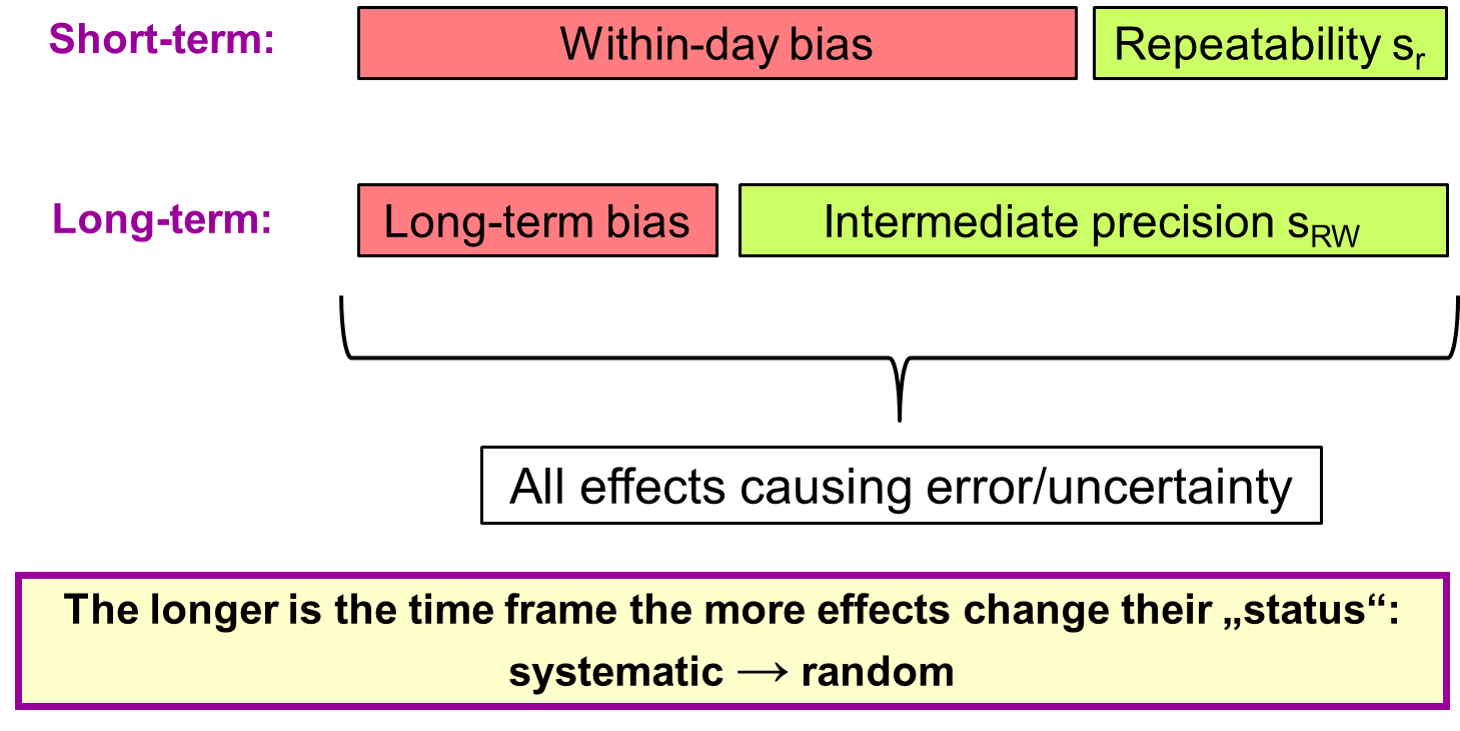
Scheme 6.2. Two ways of grouping effects that cause uncertainty (short-term and long-term).
As is explained in section 8, the two main uncertainty estimation approaches addressed in this course use the above ways as follows: The modelling (ISO GUM) approach tends to follow to the short-term view (estimating uncertainty of one concrete result on one concrete day), while the Single-lab approach (Nordtest) always follows the long-term view (estimating an average uncertainty of the procedure). See sections 8-11 for more information.
Determining repeatability and within-lab reproducibility in practice
The typical requirements for determining sr and sRW are presented in Table 6.2.
Table 6.2. Typical requirements for determining sr and sRW of an analytical procedure.
| Repeatability sr | Within-lab reproducibility sRW |
| There is a sufficient amount of a stable and homogeneous sample (control sample) | |
| The control sample has to be similar to the routinely analysed samples by analyte content and by difficulty level | |
| Sample has to be stable within a day | Sample has to be stable for months |
| Measurements with subsamples of the control sample are carried out on the same day under the same conditions | On days when the analysis procedure is used, in addition to calibrants and customer samples also a subsample of the control sample is analysed |
| The subsample of the control sample has to through all the steps of the procedure, including the sample preparation steps | |
| sr or sRW is found as standard deviation of the results obtained with subsamples of the control sample | |
When estimating the uncertainty contributions due to random effects, then it is important that a number of repeated measurements are carried out. On the other hand, if, e.g. repeatability of some analytical procedure is estimated then each repetition has to cover all steps in the procedure, including sample preparation. For this reason making extensive repetitions is very work-intensive. In this situation the concept of pooled standard deviation becomes very useful. Its essence is pooling standard deviations obtained from a limited number of measurements. The following video explains this:
Pooled standard deviation
http://www.uttv.ee/naita?id=18228
https://www.youtube.com/watch?v=xsltS41PZW0
Depending on how the experiments are planned, the pooled standard deviation can be used for calculating of either repeatability sr or within-lab reproducibility sRW. The experimental plan and calculations when finding repeatability sr are explained in the following video:
Pooled standard deviation in practice: estimating repeatability
http://www.uttv.ee/naita?id=18232
https://www.youtube.com/watch?v=DM_zf85PYic
The experimental plan and calculations when finding within-lab reproducibility sRW are explained in the following video:
Pooled standard deviation in practice: estimating within-lab long-term reproducibility
http://www.uttv.ee/naita?id=18234
https://www.youtube.com/watch?v=nPJY8HfPxNs
![]()
***
[1] It cannot be strictly defined, how long is „long-term“. An approximate guidance could be: one year is good, „several months“ (at least 4-5) is minimum. Of course it also depends on the procedure.
[2] The terms „within-lab reproducibility“ and „intermediate precision“ are synonyms. The VIM(1) prefers intermediate precision. The Nordtest handbook(5) uses within-lab reproducibility (or reproducibility within laboratory). In order to stress the importance of the „long-term“, in this course we often refer to sRW as the within-lab long-term reproducibility.
***
The slides of the presentation and the calculation files – with initial data only, as well, as with calculations performed – are available from here:

