
Brief summary: Like the individual values, the mean value calculated from them is also a random quantity. If the individual values are distributed according to the Normal distribution then the mean value calculated from them is distributed according to the Student distribution (also called as t-distribution). The properties of the t-distribution compared to the Normal distribution are explained. Importantly, the shape of the t-distribution curve depends on the number of degrees of freedom. If the number of individual values approaches infinity then the shape of the t-distribution curve approaches the Normal distribution curve.
Other distribution functions: the Student distribution
http://www.uttv.ee/naita?id=17708
https://www.youtube.com/watch?v=CWU8KM2z59I
If a measurement is repeated and the mean is calculated from the results of the single individual measurements then, just as the individual results, their mean will also be a random quantity. If the individual results are normally distributed then their mean is distributed according to the Student distribution (also known as the t-distribution). Student distribution is presented in Scheme 3.5.
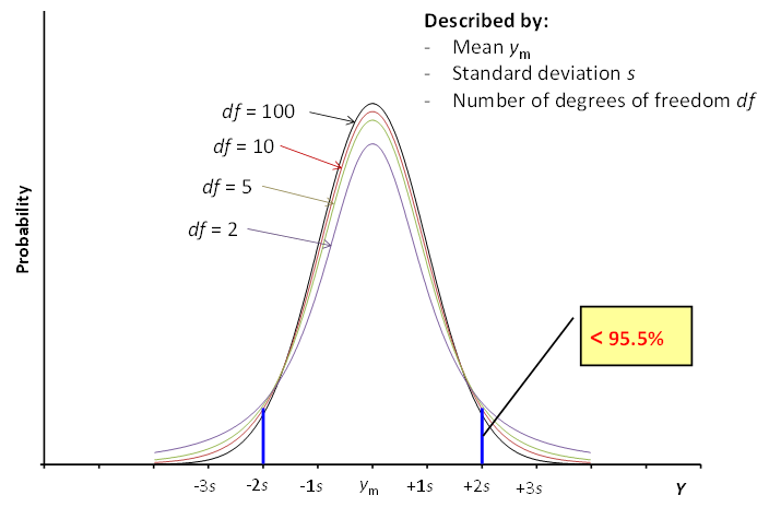
Scheme 3.5. the Student distribution.
Similarly to the normal distribution the Student distribution also has mean value ym and standard deviation s. ym is the mean value itself, [1][1] It may look strange at first sight that while the mean value ym is the only mean value we have, we immediately take it as the mean value of the distribution of mean values. However, if we had more mean values, we would anyway pool them into a single mean value (with a much higher df!) and use that value. and standard deviation is the standard deviation of the mean, calculated as explained in section 3.4. But differently from the normal distribution there is in addition a third characteristic – the number of degrees of freedom df. This number is equal to the number of repeated measurements minus one. So, the four Student distribution graphs in Scheme 3.5 correspond to 101, 11, 6 and 3 repeated measurements, respectively.
If df approaches infinity then the t-distribution approaches the normal distribution. In reality 30-50 degrees of freedom is sufficient for handling the t-distribution as the normal distribution. So, the curve with df = 100 in Scheme 3.5 can be regarded as the normal distribution curve.
The lower is the number of degrees of freedom the “heavier” are the tails of the Student distribution curve and the more different is the distribution from the normal distribution. This means that more probability resides in the tails of the distribution curve and less in the middle part. Importantly, the probabilities pictured in Scheme 3.2 for the ±1s, ±2s and ±3s ranges around the mean do not hold any more, but are all lower.
So, if a measurement result is distributed according to the t-distribution and if expanded uncertainty with predefined coverage probability is desired then instead of the usual coverage factors 2 and 3 the respective Student coefficients [2]Student coefficients (i.e. t-distribution values) for a given set of coverage probability and number of degrees of freedom can be easily obtained from special tables in statistical handbooks (use two-sided values!), from calculation or data treatment software, such as MS Excel or Openoffice Calc or from the Internet, e.g. from the address https://en.wikipedia.org/wiki/Student_distribution should be used. Measurement result can be distributed according to the Student distribution if there is a heavily dominating [3]The contributions of different uncertainty sources can be expressed numerically. This is explained in section 9.9 and the respective calculations are shown in 9.7. In this context the phrase „heavily dominating“ means that the contribution (uncertainty index) of the respective input quantity is above 75%. A type uncertainty source that has been evaluated as a mean value from a limited number of repeated measurements. More common, however, is the situation that there is an influential but not heavily dominating A-type uncertainty source. In such a case the distribution of the measurement result is a convolution [4]Convolution of two distribution functions in mathematical statistics means a combined of distribution function, which has a shape inbetween the two distribution functions that are convoluted. of the normal distribution and the t-distribution. What to do in this case is explained in section 9.8.
![]()
[1] It may look strange at first sight that while the mean value ym is the only mean value we have, we immediately take it as the mean value of the distribution of mean values. However, if we had more mean values, we would anyway pool them into a single mean value (with a much higher df!) and use that value.
[2] Student coefficients (i.e. t-distribution values) for a given set of coverage probability and number of degrees of freedom can be easily obtained from special tables in statistical handbooks (use two-sided values!), from calculation or data treatment software, such as MS Excel or Openoffice Calc or from the Internet, e.g. from the address https://en.wikipedia.org/wiki/Student_distribution
[3] The contributions of different uncertainty sources can be expressed numerically. This is explained in section 9.9 and the respective calculations are shown in 9.7. In this context the phrase „heavily dominating“ means that the contribution (uncertainty index) of the respective input quantity is above 75%.
[4] Convolution of two distribution functions in mathematical statistics means a combined of distribution function, which has a shape inbetween the two distribution functions that are convoluted.

