
Brief summary: This lecture starts by generalizing that all measured values are random quantities from the point of view of mathematical statistics. The most important distribution in measurement science – the Normal distribution – is then explained: its importance, the parameters of the Normal distribution (mean and standard deviation). The initial definitions of standard uncertainty (u ), expanded uncertainty (U ) and coverage factor (k ) are given. A link between these concepts and the Normal distribution is created.
The Normal distribution
http://www.uttv.ee/naita?id=17589
https://www.youtube.com/watch?v=N-F6leWyNZk
All measured quantities (measurands) are from the point of view of mathematical statistics random quantities. Random quantities can have different values. This was demonstrated in the lecture on the example of pipetting. If pipetting with the same pipette with nominal volume 10 ml is repeated multiple times then all the pipetted volumes are around 10 ml, but are still slightly different. If a sufficiently large number of repeated measurements are carried out and if the pipetted volumes [1]It is fair to ask, how do we know the individual pipetted volumes if the pipette always „tells“ us just that the volume is 10 ml? In fact, if we have only the pipette and no other (more accurate) measurement possibility of volume then we cannot know how much the volumes differ form each other or from the nominal volume. However, if a more accurate method is available then this is possible. In the case of pipettig a very suitable and often used more accurate method is weighing. It is possible to find the volume of the pipetted water, which is more accurate than that obtained by pipetting, by weighing the pipetted solution (most often water) and divided the obtained mass by the density of water at the temperature of water. Water is used in such experiments because the densities of water at different temperatures are very accurately known (see e.g. http://en.wikipedia.org/wiki/Properties_of_water#Density_of_water_and_ice). are plotted according to how frequently they are encountered then it becomes evident that although random, the values are still governed by some underlying relationship between the volume and frequency: the maximum probability of a volume is somewhere in the range of 10.005 and 10.007 ml and the probability gradually decreases towards smaller and larger volumes. This relationship is called distribution function (the more exact term is probability density function).
There are numerous distribution functions known to mathematicians and many of them are encountered in the nature, i.e. they describe certain processes in the nature. In measurement science the most important distribution function is the normal distribution (also known as the Gaussian distribution). Its importance stems from the so-called Central limit theorem. In a simplified way it can be worded for measurements as follows: if a measurement result is simultaneously influenced by many uncertainty sources then if the number of the uncertainty sources approaches infinity then the distribution function of the measurement result approaches the normal distribution, irrespective of what are the distribution functions of the factors/parameters describing the uncertainty sources. In reality the distribution function of the result becomes indistinguishable from the normal distribution already if there are 3-5 (depending on situation) significantly contributing [2]Significantly cointributing uncertainty sources are the important uncertainty sources. We have already qualitatively seen in section 2 that different uncertainty sources have different „importance“. In the coming lectures we will also see how the „importance“ of an uncertainty source (its uncertainty contribution) can be quantitatively expressed. uncertainty sources. This explains, why in so many cases measured quantities have normal distribution and why most of the mathematical basis of measurement science and measurement uncertainty estimation is based on the normal distribution.
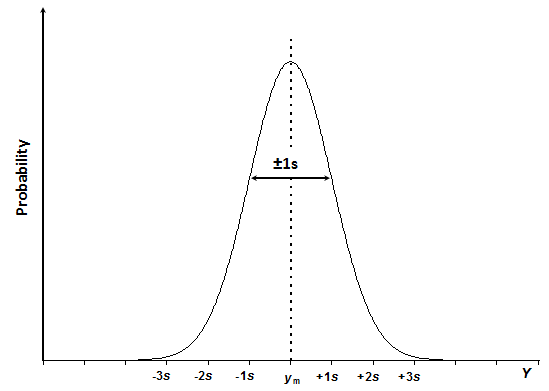
Scheme 3.1. The normal distribution curve of quantity Y with mean value ym and standard deviation s.
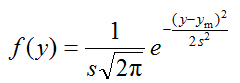
The normal distribution curve has the bell-shaped appearance (Scheme 3.1), and is expressed by equation 3.1:
|
(3.1) |
In this equation f ( y ) is the probability (or more exactly – probability density) that the measurand Y has value y. ym is the mean value of the population and s is the standard deviation of the population. ym characterizes the position of the normal distribution on the Y axis, s characterizes the width (spread) of the distribution function, which is determined by the scatter of the data points. The mean and standard deviation are the two parameters that fully determine the shape of the normal distribution curve of a particular random quantity. The constants 2 and \(\pi\) are normalization factors, which are present in order to make the overall area under the curve equal to 1.
The word “population” here means that we would need to do an infinite number of measurements in order to obtain the true ym and s values. In reality we always operate with a limited number of measurements, so that the mean value and standard deviation that we have from our experiments are in fact estimates of the true mean and true standard deviation. The larger is the number of repeated measurements the more reliable are the estimates. The number of parallel measurements is therefore very important and we will return to it in different other parts of this course.
The normal distribution and the standard deviation are the basis for definition of standard uncertainty. Standard uncertainty, denoted by u, is the uncertainty expressed at standard deviation level, i.e., uncertainty with roughly 68.3% coverage probability (i.e. the probability of the true value falling within the uncertainty range is roughly 68.3%). The probability of 68.3% is often too low for practical applications. Therefore uncertainty of measurement results is in most cases not reported as standard uncertainty but as expanded uncertainty. Expanded uncertainty, denoted by U, is obtained by multiplying standard uncertainty with a coverage factor,[3]This definition of expanded uncertainty is simplified. A more rigorous definition goes via the combined standard uncertainty and is introduced in section 4.4. denoted by k, which is a positive number, larger than 1. If the coverage factor is e.g. 2 (which is the most commonly used value for coverage factor) then in the case of normally distributed measurement result the coverage probability is roughly 95.5%. These probabilities can be regarded as fractions of areas of the respective segments from the total area under the curve as illustrated by the following scheme:
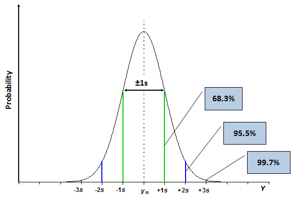
Scheme 3.2. The same normal distribution curve as in Scheme 3.1 with 2s and 3s segments indicated.
Since the exponent function can never return a value of zero, the value of f ( y ) (eq 3.1) is higher than zero with any value of y. This is the reason why uncertainty with 100% coverage is (almost) never possible.
It is important to stress that these percentages hold only if the measurement result is normally distributed. As said above, very often it is. There are, however, important cases when measurement result is not normally distributed. In most of those cases the distribution function has “heavier tails”, meaning, that the expanded uncertainty at e.g. k = 2 level will not correspond to coverage probability of 95.5%, but less (e.g. 92%). The issue of distribution of the measurement result will be addressed later in this course.
![]()
***
[1] It is fair to ask, how do we know the individual pipetted volumes if the pipette always „tells“ us just that the volume is 10 ml? In fact, if we have only the pipette and no other (more accurate) measurement possibility of volume then we cannot know how much the volumes differ form each other or from the nominal volume. However, if a more accurate method is available then this is possible. In the case of pipettig a very suitable and often used more accurate method is weighing. It is possible to find the volume of the pipetted water, which is more accurate than that obtained by pipetting, by weighing the pipetted solution (most often water) and divided the obtained mass by the density of water at the temperature of water. Water is used in such experiments because the densities of water at different temperatures are very accurately known (see e.g. http://en.wikipedia.org/wiki/Properties_of_water#Density_of_water_and_ice).
[2] Significantly cointributing uncertainty sources are the important uncertainty sources. We have already qualitatively seen in section 2 that different uncertainty sources have different „importance“. In the coming lectures we will also see how the „importance“ of an uncertainty source (its uncertainty contribution) can be quantitatively expressed.
[3] This definition of expanded uncertainty is simplified. A more rigorous definition goes via the combined standard uncertainty and is introduced in section 4.4.

